Objectives
This lab introduces techniques of picking the state representation \( X\in \mathbb{R}^{n} \), control input representation \( u \in \mathbb{R}^l \), observation \( o \in \mathbb{R}^m \) and characterizing these matrices:
\( A \in \mathbb{R}^{n\times n}\): state transition matrix;
\( B \in \mathbb{R}^{l\times n} \): control input matrix;
\( C \in \mathbb{R}^{m\times n} \): observation matrix;
as well as other noise matrices. Finally, we will be able to predict the ToF reading in addition to the slow update of the ToF sensor.
Task 1: Estimate Drag and Momentum
How to Calculate Params
To characterize the state transition matrix and control input matrix, we can use Newton's Law to solve the dynamics equations.Let the state representation be \( X = \left[ \begin{matrix} v \\ a \end{matrix} \right] \) (where \( v,a \) are the velocity and acceleration), the control input be \( u \in \mathbb{R} \).
Thus we have the following equations:
\( \begin{cases} v' = v \\ F_{traction} - F_{drag} = m\cdot a \end{cases} \)
Using Newton's Law, let the PWM value approximate the traction force (with approximation for the drag coefficient \( d \)), we have: \( u - d\cdot v = m\cdot a \to a = \frac{1}{m}u - \frac{d}{m}v \)
Therefore, in the steady state, the prediction step of the Kalman Filter can be written as: \( \hat{X} = \left[ \begin{matrix} \hat{v} \\ \hat{a} \end{matrix} \right] = \left[ \begin{matrix} 1 & 0 \\ -\frac{d}{m} & 0 \end{matrix} \right]\cdot \left[ \begin{matrix} v \\ a \end{matrix} \right] + \left[ \begin{matrix} 0 \\ \frac{1}{m} \end{matrix} \right] \cdot u \)
At steady state, we have \( a = 0 \) so that we have \( d = \frac{u}{v_s} \) (where \( v_s \) is the steady state speed).
Using first order time invariant system to characterize the dynamics of the car, we have:
\( \tau\frac{dv(t)}{dt} + v(t) = Ku(t) \to \frac{dv(t)}{dt} + \frac{1}{\tau} v(t) = \frac{K}{\tau}u(t) \), where \( a(t) = \frac{dv(t)}{dt} \).
Compare the above equation with the motion formula, we have \( \tau = \frac{m}{d}, K = \frac{1}{d} \). Based on the inverse Laplacian transformation, we can obtain the response of a 1-st order system's response to a Unit Step input: \( y(t) = 1 - e^{-\frac{1}{\tau}t} = 1 - e^{-\frac{d}{m}t} \). (Computation Reference (in Chinese))
Using 90% rise time, we have: \( 0.9 = 1 - e^{-\frac{d}{m}t_{0.9rise}} \to -\frac{d}{m}t_{0.9rise} = \log(0.1) \to m = - \frac{d}{\log(0.1)}t_{0.9rise} \)
Measure the Steady State Speed and Rise Time
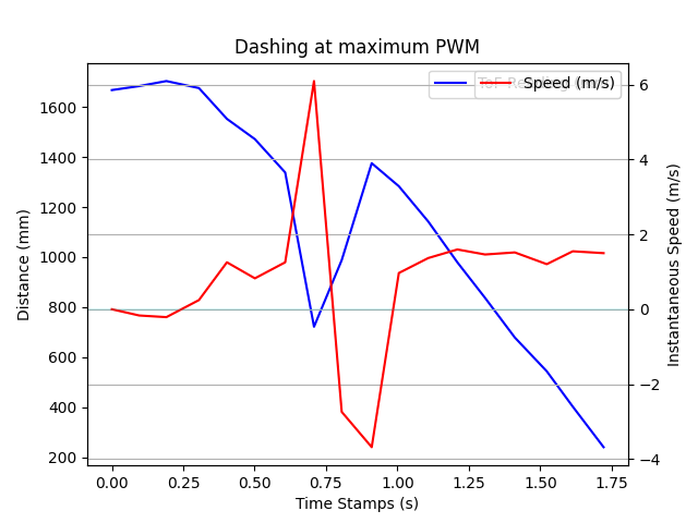
Observing the result above, we can get an average steady speed at \( v_s = 1.8 m/s \), 90% rise time is \( t_{0.9rise} = 0.9\times 1.25 = 1.125s \). The car was driving at PWM = 183, so \( u = 183/255 \). Thus, \( d = \frac{u}{v_s} = \frac{183}{1.125\times 255} \approx 0.3986928104575163 \).
Plugging \( d = 0.3986928104575163 \) into \( m =- \frac{d}{\log(0.1)}t_{0.9rise} \), we have \( m = -\frac{0.3986\times 1.125}{-2.3026} = 0.1947 \)
Task 2: Initialize Kalman Filter
Having those params, we can directly initialize the KF filter matrices along with defining the state as [distance, speed].
\( \left[ \begin{matrix} x \\ \dot{x} \end{matrix} \right] = \left[ \begin{matrix} 1 & dt \\ 0 & 1 - dt\cdot\frac{d}{m} \end{matrix}\right]\cdot \left[ \begin{matrix} x \\ \dot{x} \end{matrix} \right] + \left[ \begin{matrix} 0 \\ dt\cdot\frac{1}{m} \end{matrix} \right]\cdot u \)
The Kalman Filter params can be stored using a python object. Due to the unfixed time interval between ToF data, the A and B matrices below remain updated in real-time.
                                        u = 183/255  # maxPWM count
                                        vel = 1.8  # m/s
                                        d = u/vel
                                        dt = 1.125  # 90% rise time, sec. 1.125.
                                        m = -dt*d/(np.log(0.1))

                                        class KF():
                                            def __init__(self, d, m, sigma1, sigma2, sigma3):
                                                self.d = d
                                                self.m = m
                                                self.R = np.diag([sigma1 ** 2, sigma2 ** 2])
                                                self.Q = np.array([sigma3 ** 2])
                                                self.C = C = np.array([[1],
                                                                       [0]])
                                            def A(self, dtloop):
                                                A = np.array([[1, dtloop],
                                                              [0, 1 - dtloop*self.d/self.m]])
                                                return A
                                            def B(self, dtloop):
                                                B = np.array([[0],
                                                              [dtloop/self.m]])
                                                return B
The covariance matrix characterizes the noise of a certain state or measurement relative to itself or other states / measurements. For now, we assume that the noise between different state entries and different measurements entries is not correlated. So that we obtain two diagnal matrices as those noise matrices. Empirically we choose \( \sigma_1 = 0.05m, \sigma_2 = 0.05m/s, \sigma_3 = 0.02m \). Since the experiment range is 0~1m, the sensor readings mostly fall into the range between the real value \( \pm 3\times\sigma_3 = \pm 3\times 0.02m = \pm 6cm \), according to the "3\( \sigma \)" rule in statistics. Actually the 12cm error range for the ToF is quite excessive, since the VL53L0X manual gives a 1-\(\sigma\) value = 2.5~3.5mm at the long range mode (refer to the manual page 11). But we'll see that the Kalman Filter is still robust even given excessive noise.
Task 3: Implement and Test the Kalman Filter in Jupyter
Now we use the following code to implement the Kalman Filter updates.
                                        # Kalman Filter Update
                                        KFStates = []
                                        KFSigmas = []
                                        myKF = KF(d, m, 0.05, 0.05, 0.02)
                                        Sigma = np.diag([0.001, 0.001])
                                        KFSigmas.append(Sigma)
                                        KFPreds = []
                                        for i, oneData in enumerate(data):
                                            # prediction step
                                            oneData = oneData.copy()
                                            oneData[1] *= (-0.001)  # convert to nagative meters.
                                            oneData[0] *= 0.001 # convert to seconds.
                                            oneData[2] = oneData[2] / 255
                                            if i == 0:
                                                lastTime = oneData[0]
                                                X = np.array([[oneData[1]],
                                                              [oneData[2]]])
                                                KFStates.append(X)
                                                KFPreds.append(X)
                                                continue
                                            dt = (oneData[0] - lastTime)
                                            # print(dt)
                                            lastTime = oneData[0]
                                            Xpred = myKF.A(dt).dot(X) + myKF.B(dt)*(oneData[2])  # mean update.
                                            KFPreds.append(Xpred)
                                            SigmaPred = myKF.A(dt).dot(Sigma).dot(myKF.A(dt).T) + myKF.R  # covariance update.
                                            # calculate Kalman Gain.
                                            inv = np.linalg.inv(myKF.C.T.dot(SigmaPred).dot(myKF.C) + myKF.Q)  # 1x1
                                            K = SigmaPred.dot(myKF.C).dot(inv)  # 2x1
                                            # update state belief.
                                            X = Xpred + K.dot(oneData[1] - myKF.C.T.dot(Xpred))  # convert observation to meters.
                                            KFStates.append(X)
                                            # update the uncertainty.
                                            Sigma = (np.eye(2) - K.dot(myKF.C.T)).dot(SigmaPred)
                                            KFSigmas.append(Sigma)
We use the following code to visualize the predictions in comparison with the real ToF readings. The RED Dotted Line indicates the curve of final predictions of the KF. The initial belief (before incorporating observation data) array is also plotted in the diagram.
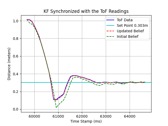
We use the following code to calculate the overall average error between prediction (updated belief) and real ToF readings. The average error is 0.00300120719728453 m.
error = np.sum(np.abs(data[:, 1] / 1000 + KFStates[:, 0])) / 50
Additional Task: State Estimation In Addition to ToF
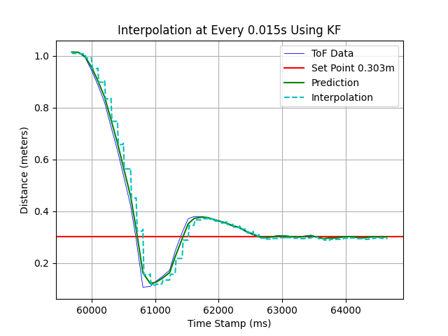
Sometimes the ToF readings come at a disappointing rate, we need to update the state of robot at a faster speed to make safe and timely decisions. The following code simulates a senario that the ToF readings come at around every 0.1s (which is also the actual rate using long-range mode). The Interpolation interval is set to 15ms, which is adjustable.
                                    # Kalman Filter Update
                                    KFStates = []
                                    KFSigmas = []
                                    myKF = KF(d, m, 0.03, 0.03, 0.02)
                                    Sigma = np.diag([0.001, 0.001])
                                    KFSigmas.append(Sigma)
                                    KFPreds = []
                                    KFPredsStamps = []
                                    dtInt = 15/1000  # sec.

                                    for i, oneData in enumerate(data):
                                        # prediction step
                                        oneData = oneData.copy()
                                        oneData[1] *= (-0.001)  # convert to nagative meters.
                                        oneData[0] *= 0.001 # convert to seconds.
                                        oneData[2] = oneData[2] / 255
                                        if i == 0:
                                            lastTime = oneData[0]
                                            X = np.array([[oneData[1]],
                                                          [oneData[2]]])  # store the initial PWM as the initial speed.
                                            KFStates.append(X)
                                            KFPreds.append(X)
                                            KFPredsStamps.append(lastTime)
                                            lastControl = oneData[2]
                                            continue

                                        # interpolation
                                        while(lastTime + dtInt < oneData[0]):  # no new data.
                                            lastTime += dtInt
                                            dt = dtInt
                                            Xpred = myKF.A(dt).dot(X) + myKF.B(dt)*(lastControl)  # mean update.
                                            KFPreds.append(Xpred)
                                            KFPredsStamps.append(lastTime)
                                            SigmaPred = myKF.A(dt).dot(Sigma).dot(myKF.A(dt).T) + myKF.R  # covariance update.

                                        dt = oneData[0] - lastTime
                                        lastTime = oneData[0]
                                        Xpred = myKF.A(dt).dot(X) + myKF.B(dt)*(oneData[2])  # mean update.
                                        KFPreds.append(Xpred)
                                        KFPredsStamps.append(lastTime)
                                        SigmaPred = myKF.A(dt).dot(Sigma).dot(myKF.A(dt).T) + myKF.R  # covariance update.
                                        # calculate Kalman Gain.
                                        inv = np.linalg.inv(myKF.C.T.dot(SigmaPred).dot(myKF.C) + myKF.Q)  # 1x1
                                        # print("inv", inv)
                                        K = SigmaPred.dot(myKF.C).dot(inv)  # 2x1
                                        # print("K:\n", K)
                                        # update state belief.
                                        X = Xpred + K.dot(oneData[1] - myKF.C.T.dot(Xpred))  # convert observation to meters.
                                        # print("X: ", X)
                                        KFStates.append(X)
                                        # update the uncertainty.
                                        Sigma = (np.eye(2) - K.dot(myKF.C.T)).dot(SigmaPred)
                                        KFSigmas.append(Sigma)
                                        lastControl = oneData[2]
The result with 6x interpolation is shown below.
There are also other interpolation rates being tested.
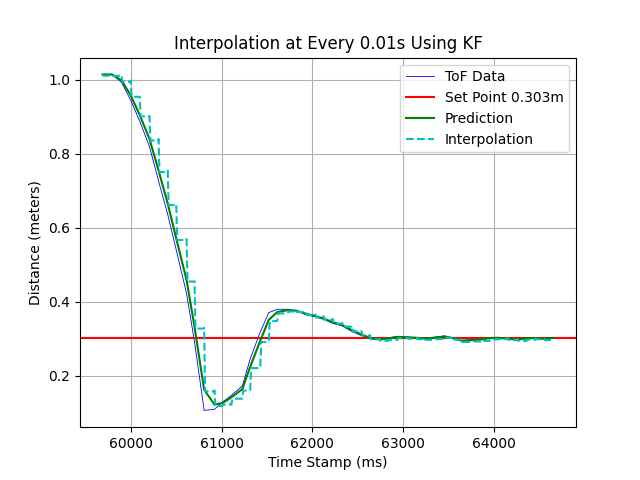
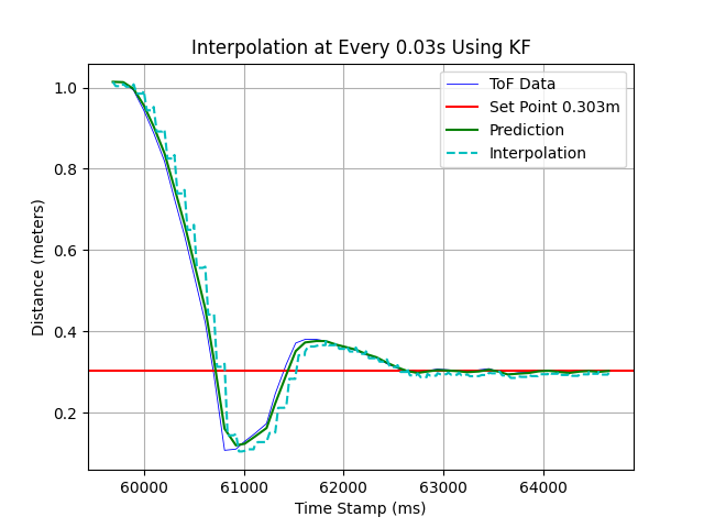
Observing the above figures, we may extrapolate that the higher interpolation frequency yeilds better convergence of initial beliefs when the system converges.
Additional PCB Design for the Dual Motor Driver
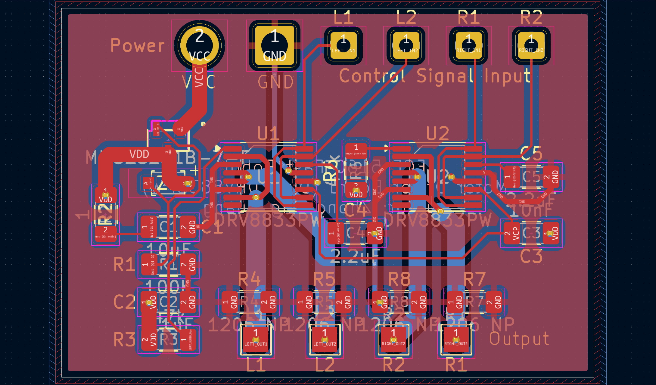
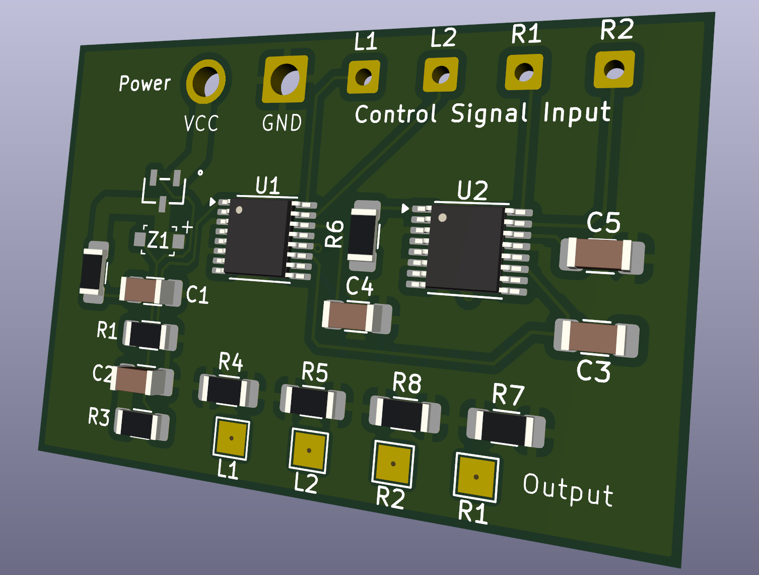
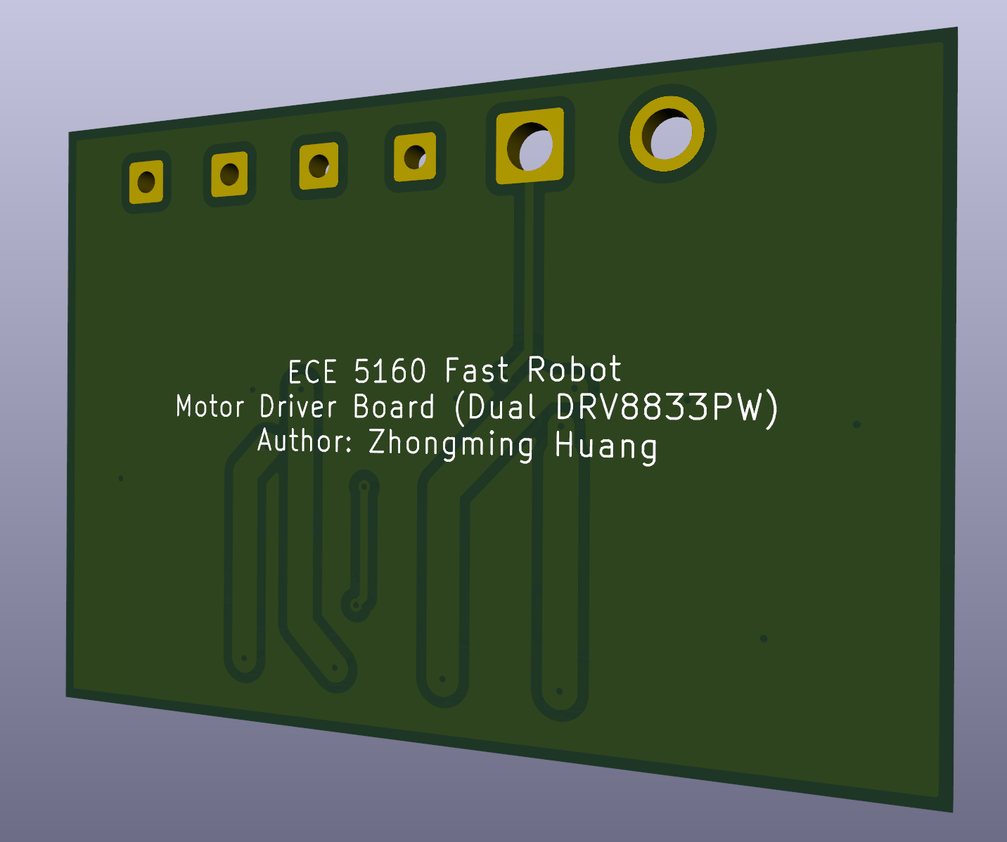
Due to the frequent mulfunctions rising from the two motor drivers, I designed a PCB board to hold the two drivers with optimized power output wiring. The board's order has been placed and I'll solder components onto it if there's available time.
THE END